In previous articles, we looked at performing machine learning tasks such as forecasting and anomaly detection directly within ClickHouse using only SQL.
Though we demonstrated successful results with those examples, there are still many machine learning tasks where we realistically need to break out of SQL and into an imperative programming language and inference environment.
In this circumstance, we like to use AWS SageMaker, which is a component of AWS which can be used for the full machine learning lifecycle from development through to deployment.
Of course, we will back SageMaker with ClickHouse Cloud, using it as a high performance datastore to support the ML lifecycle.
Why ClickHouse Is A Good Fit For Machine Learning
Even though we are making use of SageMaker and working within the AWS ecosystem, ClickHouse Cloud still makes an excellent datastore when developing machine learning models. For instance, it makes a great repository for training data, for the results of experiments, for feature engineering and for storing machine learning observability data.
We explain this in more detail in this article.
AWS Sagemaker Environment
For this demo, we are going to use the classic AWS SageMaker notebook instance. This is a hosted Jupyter Notebook service which offers the familiar notebook based interface and the ability to execute Python code on an attached EC2 server.
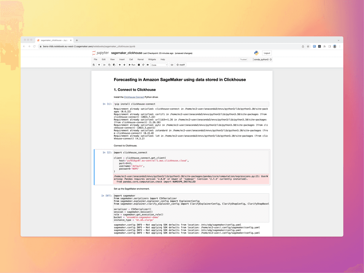
For our interactions with ClickHouse, we will use the ClickHouse connect Python library which can be installed through the Jupyter notebook.
Even though we are in this simple notebook environment, SageMaker is a very fully featured product which includes a number of features such as data labelling, training, testing, deployments, hyperparameter optimisation and more.
Dataset and Scenario
We are going to use a subset of the "Metro Interstate Traffic Volume" dataset from the UCI Machine Learning Repository, which we will load into a table in ClickHouse.
The dataset contains the hourly time series of westbound traffic volume in Minneapolis ATR station 301 route I-94. The data was recorded over 6 years from the beginning of October 2012 to the end of September 2018.
Our aim will be to take this data and use it to train a predictive model. The model will then be exposed for "real-time inference", whereby we present new data to the endpoint and ask it to synchronously make predictions about the next hour of traffic.
We will use the majority of the data between 2012 to 1st September 2018 for training. We will then test the model using data between 1st September 2018 and 31st September 2018.
Our source data has the following simple structure:
SELECT *
FROM traffic
LIMIT 10

Query id: 2d979087-2381-4ba0-b740-839b4b430997

┌───────────date_time─┬─traffic_volume─┐
│ 2012-10-02 09:00:00 │           5545 │
│ 2012-10-02 10:00:00 │           4516 │
│ 2012-10-02 11:00:00 │           4767 │
│ 2012-10-02 12:00:00 │           5026 │
│ 2012-10-02 13:00:00 │           4918 │
│ 2012-10-02 14:00:00 │           5181 │
│ 2012-10-02 15:00:00 │           5584 │
│ 2012-10-02 16:00:00 │           6015 │
│ 2012-10-02 17:00:00 │           5791 │
│ 2012-10-02 18:00:00 │           4770 │
└─────────────────────┴────────────────┘

10 rows in set. Elapsed: 0.058 sec. Processed 8.19 thousand rows, 65.54 KB (141.30 thousand rows/s., 1.13 MB/s.)
Peak memory usage: 966.16 KiB.
The data has the following distribution over time:
SELECT
    toStartOfYear(date_time) AS year,
    count(*)
FROM traffic
GROUP BY year

Query id: a3fafc5f-bd9a-4ca4-9a3a-4642418396ff

┌───────year─┬─count()─┐
│ 2012-01-01 │    2103 │
│ 2013-01-01 │    7294 │
│ 2014-01-01 │    4501 │
│ 2015-01-01 │    3593 │
│ 2016-01-01 │    7838 │
│ 2017-01-01 │    8713 │
│ 2018-01-01 │    6533 │
└────────────┴─────────┘

7 rows in set. Elapsed: 0.003 sec. Processed 40.58 thousand rows, 162.30 KB (11.85 million rows/s., 47.39 MB/s.)
Peak memory usage: 49.52 KiB.
Data Preparation
We will begin by loading the data directly from ClickHouse into a dataframe:
data = client.query_df('select * from traffic')
We can then conduct some exploratory analysis to get a feel for the dataset:
daily_means = data.groupby(by=data['date_time'].dt.weekday)['traffic_volume'].mean()
daily_means
Outputs:
date_time
0    3313.560547
1    3534.717285
2    3608.276123
3    3653.914795
4    3674.777588
5    2822.564697
6    2426.249512
In order to forecast the traffic volume over a given hour, we use as features the traffic volume during the previous hour, the hour of the day and the day of the week. These are extracted from the date_time column.
data['previous_traffic_volume'] = data['traffic_volume'].shift(1)
data['hour'] = data['date_time'].dt.hour
data['weekday'] = data['date_time'].dt.weekday
data.dropna(inplace=True, ignore_index=True)
As discussed, we will set aside the last month of data for testing, and we use all the remaining data for training.
train_data = data[data['date_time'] < '2018-09-01 00:00:00']
test_data = data[data['date_time'] >= '2018-09-01 00:00:00']
Feature Store
At this point, data could also be serialized into some "feature store" tables within ClickHouse so they are available for other team members or for the development of other models. This also helps with reproducability as we effectively have a reusable record of the data used to train and test the model. Again ClickHouse has a strong proposition in this area:
client.command('''
create or replace table traffic_feature_store (
    date_time DateTime,
    previous_traffic_volume Float32,
    hour Int32,
    weekday Int32,
) ENGINE MergeTree ORDER BY date_time
''')
client.insert_df('traffic_feature_store', test_data.drop(labels=['traffic_volume'], axis=1))
Save The Data In S3
We will use the CatBoost SageMaker built-in algorithm for the forecast which enhances the Gradient Boosting Decision Tree (GBDT) algorithm.
Because it's a built-in algorithm, it requires training data to be saved in S3 in CSV format. If we were to develop our own model in our own container, we could integrate directly with ClickHouse to access training data directly.
We drop the date_time column before saving the training dataset in S3, as this column is not used as a feature. Note that, after dropping the date_time column, the target variable traffic_volume is moved to the first column, putting it into the structure required by the algorithm.
_ = session.upload_string_as_file_body(
    body=train_data.drop(labels=['date_time'], axis=1).to_csv(index=False, header=False),
    bucket=bucket,
    key='train/data.csv'
)
The algorithm also requires a JSON file with the column indices of the categorical features (in our case, hour and weekday) to be saved in S3 together with the training data. After dropping the date_time column, the hour and weekday columns have indices 2 and 3 respectively.
_ = session.upload_string_as_file_body(
    body=json.dumps(dict(cat_index_list=[2, 3])),
    bucket=bucket,
    key='train/categorical_index.json'
)
Model Training
With the CSV and JSON metadata prepared, we are now ready to train the CatBoost model:
model_id = 'catboost-regression-model'
model_version = '*'

train_image_uri = sagemaker.image_uris.retrieve(
    region=None,
    framework=None,
    model_id=model_id,
    model_version=model_version,
    image_scope='training',
    instance_type=instance_type
)

train_source_uri = sagemaker.script_uris.retrieve(
    model_id=model_id,
    model_version=model_version,
    script_scope='training',
)

train_model_uri = sagemaker.model_uris.retrieve(
    model_id=model_id,
    model_version=model_version,
    model_scope='training',
)

estimator = sagemaker.estimator.Estimator(
    role=role,
    image_uri=train_image_uri,
    source_dir=train_source_uri,
    model_uri=train_model_uri,
    instance_count=1,
    instance_type=instance_type,
    max_run=3600,
    output_path=f's3://{bucket}/output',
    entry_point='transfer_learning.py',
)

estimator.fit({'training': f's3://{bucket}/train'})
Model Deployment
After the model has been trained, we can deploy it to a Sagemaker real-time endpoint. This makes it available as a running process which can execute against for inference. These endpoints are designed for low latency and also offer auto-scaling.
deploy_image_uri = sagemaker.image_uris.retrieve(
    region=None,
    framework=None,
    image_scope='inference',
    model_id=model_id,
    model_version=model_version,
    instance_type=instance_type,
)

deploy_source_uri = sagemaker.script_uris.retrieve(
    model_id=model_id,
    model_version=model_version,
    script_scope='inference',
)

predictor = estimator.deploy(
    initial_instance_count=1,
    instance_type=instance_type,
    entry_point='inference.py',
    image_uri=deploy_image_uri,
    source_dir=depl
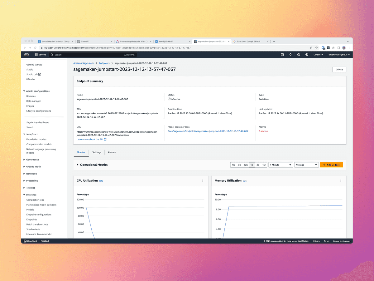
After deployment, the real time endpoint can then be viewed in the SageMaker console, where metrics about how it is being used can also be observed:
Model Inference
In a real application or stream processing scenario, we would invoke the endpoint periodically or on demand to obtain the traffic forecasts for the next hour.
To reproduce this scenario, we iterate over the rows of the test dataset, and invoke the endpoint with the data in each row in order to predict the next observation.
We will begin by creating a new table in ClickHouse for storing the forecasts:
client.command('''
create or replace table traffic_real_time_forecasts (
    date_time DateTime,
    traffic_volume_forecast Float32,
) ENGINE MergeTree ORDER BY date_time
''')
Next, we iterate over the test dataset and call the endpoint for each row, saving the forecasted results into the ClickHouse table.
# list the hours in the test set
timestamps = pd.date_range(start='2018-09-01 00:00:00', end='2018-09-30 23:00:00', freq='H')

# loop across the hours in the test set
for timestamp in tqdm(timestamps):

    # get the model inputs from the Clickhouse feature store table
    inputs = client.query(f"select previous_traffic_volume, hour, weekday from traffic_feature_store where date_time = toDateTime('{timestamp}')")

    # serialize the model inputs
    payload = serializer.serialize(inputs.result_rows)

    # invoke the model endpoint
    response = session.sagemaker_runtime_client.invoke_endpoint(
        EndpointName=predictor.endpoint_name,
        ContentType='text/csv',
        Body=payload
    )

    # deserialize the model outputs
    prediction = deserializer.deserialize(response['Body'], 'text/csv')['prediction'][0]

    # save the model outputs in the Clickhouse real-time forecasts table
    client.insert(
        'traffic_real_time_forecasts',
        data=[[timestamp, prediction]],
        column_names=['date_time', 'traffic_volume_forecast']
    )
Model Evaluation
Having produced our forecasts, we would now like to evaluate the performance of the model by comparing it against the test dataset.
We do this by calculating the root mean squared error (RMSE) and the mean absolute percentage error (MAPE).
Our results were 318 and 13% respectively. This means our observations are approximately 87% accurate which is reasonably strong performance considering the seasonality of the dataset and the changing traffic patterns throughout the day.
RMSE:
mean_squared_error(
    y_true=test_data['traffic_volume'].values,
    y_pred=real_time_forecasts['traffic_volume_forecast'].values,
    squared=False
)
Outputs:
318.3038
MAPE:
mean_absolute_percentage_error(
    y_true=test_data['traffic_volume'].values,
    y_pred=real_time_forecasts['traffic_volume_forecast'].values
)
Outputs:
0.13059244
Note that we could also have calculated these performance metrics directly within ClickHouse as we did in our forecasting and anomaly detection examples.
Using The Forecasts
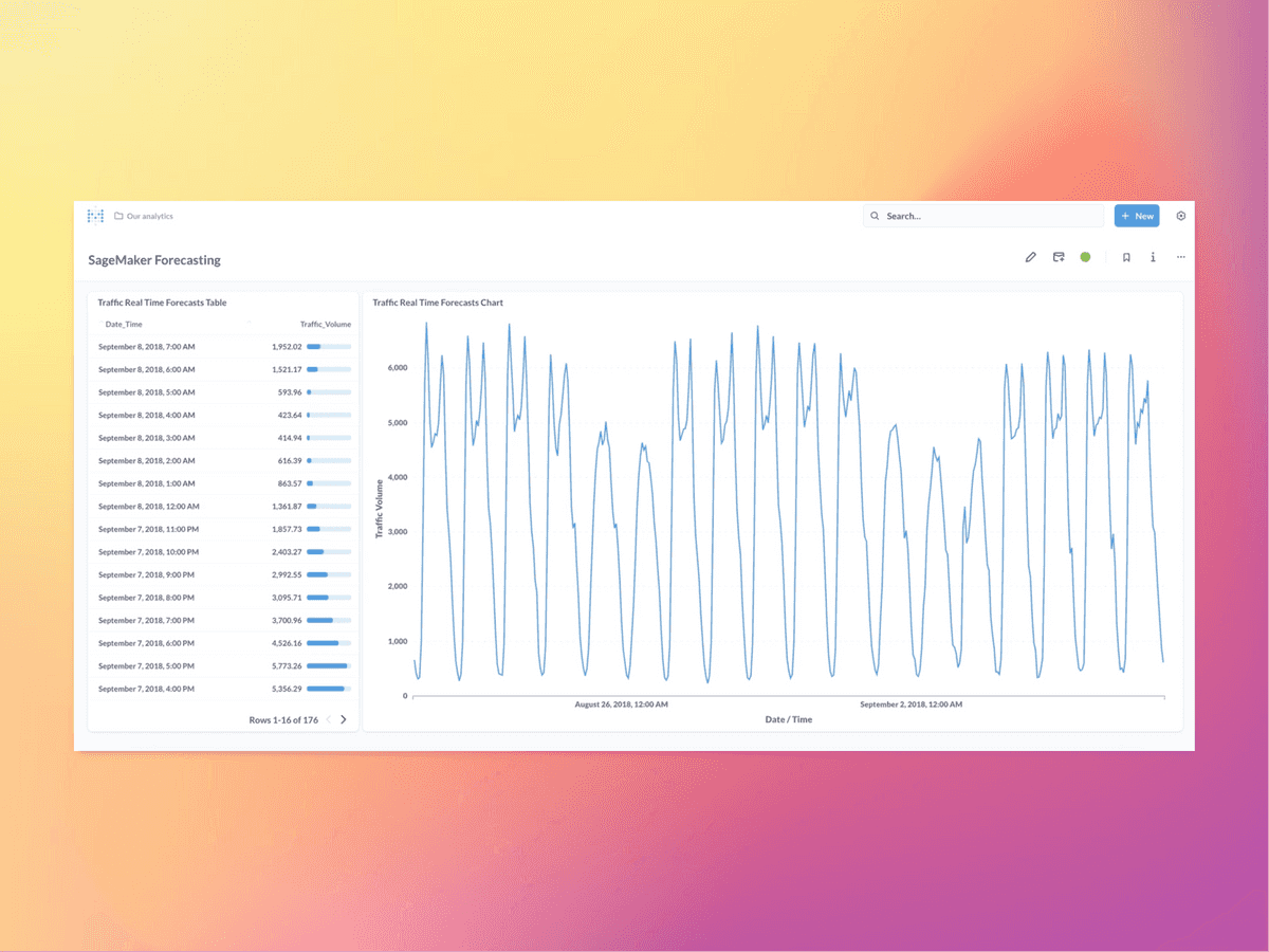
Though we deployed this model as a real-time endpoint, now we have the forecast data accruing within ClickHouse, we can easily use it for other purposes. For instance, we may simply wish to render our forecasts on a dashboard or embed them in a user facing application.
Below, we have rendered the results of our forecast iterations on a Metabase dashboard which is connected to the results stored in ClickHouse:
Observability
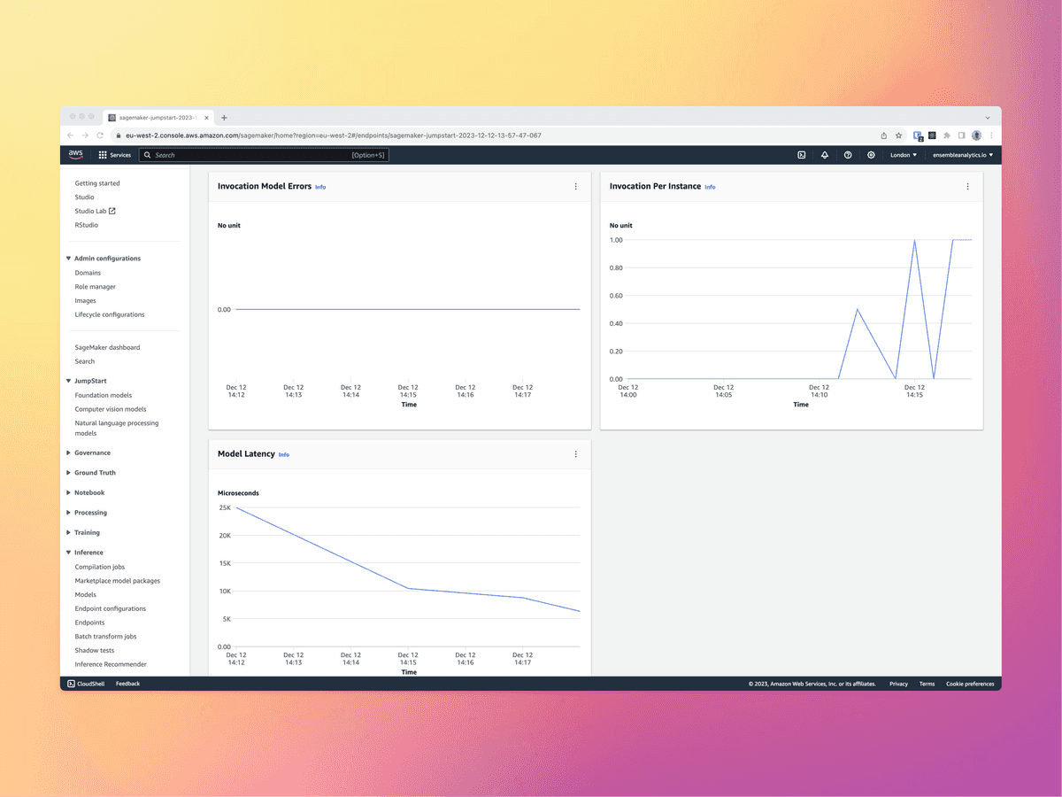
AWS SageMaker has a good story around observability and monitoring how models are being invoked in production. This includes metrics such as CPU and memory, latency, number of invocations and errors:
This said, it may be worth going beyond this and capturing more granular data about how our models are being used. At scale, machine learning models can create an enormous amount of inference data which we may wish to retain and use as we continue the development of the models. Again, ClickHouse is the ideal location to store this.
One route for doing this would be to log invocations using the "model monitor" feature of SageMaker. This would write logs of the invocation to S3, which could then be accessed as external tables within ClickHouse and potentially be bought into tools such as Grafana.
The model monitor is configured like so:
from sagemaker.model_monitor import DataCaptureConfig

data_capture_config = DataCaptureConfig(
    enable_capture=True,
    sampling_percentage=100,
    destination_s3_uri='s3://path/for/data/capture'
)
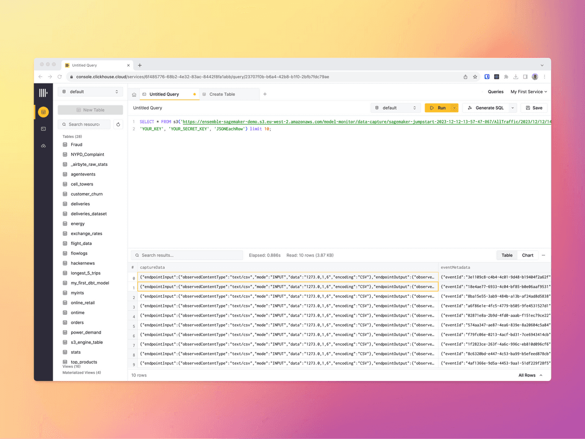
By default, the inputs and outputs will be logged as JSON files in S3. These can then be queried in ClickHouse using the S3 table function or S3 table engine within ClickHouse. This effectively gives us live observability of the machine learning model with SQL based observability.
SELECT * FROM s3('https://ensemble-sagemaker.s3.eu-west-2.amazonaws.com/model-monitor/data-capture/sagemaker-jumpstart-2023-12-12-13-57-47-067/AllTraffic/2023/12/12/14/*.jsonl',
'YOUR_KEY', 'YOUR_SECRET_KEY', 'JSONEachRow') limit 10;
Outputs:
Conclusion
In this article we have demonstrated how we can use AWS SageMaker to implement a simple forecasting function based on the CatBoost built-in algorithm.
We have demonstrated a degree of integration with ClickHouse, using it as the initial store for the training data, as a feature store, as the store for the results of our inference and to support model observability.
We believe that this represents a powerful combination of tools and workflow, and hopefully we have made the case that supporting your machine learning lifecycle with ClickHouse has value.
Sample Notebook
A notebook describing the full process can be found in this repo.


